Three key COVID-19 indicators to curb a potential of 20 million human fatality

Apr 16, 2020
-
J. Bughin

Table of Contents:

Introduction
An history of scary viruses
What about influenza?
The three key figures that matter for COVID-19
The emerging best guess picture for COVID-19: potential without control of up to 20 million fatalities worldwide
A coordinated global action plan may be required

1. Introduction

March 2

Today’s major headline across the globe is the spread of the new coronavirus, COVID-19, soon to affect 100,000s of individual in the coming weeks since its start by December 2019, presumably from a market in the Hubei province, China. There is large concern among the population as to how COVID-19 will unfold, given health and economic consequences. The number of Google searches increased 100-fold in the last six weeks across the planet, and many stock marketplaces went down significantly with losses of more than 10% from their peak during the last week of February, as a likely fear that the COVID-19 may become a major pandemic.

In the first of what I hope to be a working series around COVID-19, I review the evidence around the virus deployment. In this article, I focus on three main indicators whose current ranges may imply a most probable case of a world pandemic with a power to be killing up to 20 million humans in the absence of any interventions:

Fatality rate: Enough to take notice (with a range between 0.5% and 2%).
Reproduction rate: More a wide pandemic than a niche (adjusted $R_0$ between 1.3 to 2, with mean at 1.9)
Variance of reproduction: Super-spreaders likely the rule (top 20% accounts for between 40% to 70% of secondary infections).

Of course, figures are early and may change, for the better or for the worse. The better may evidently come from an active and rapid management of actions at global level to curb those three main indicators of the COVID-19. Such actions are today patchy; a more synchronized way to reflect our globalized world is a more promising route to date to curb the pandemics and re-route the world for a better life and growth economics.

2. A history of scary viruses

Back to Table of Contents

Viruses and their outbreaks are part of our life. But some outbreaks can become significant, mutating to pandemics with extensive and exponential attacks on human society, causing major societal disruptions. The plague of Athens caused by typhus started by about 430 years BCE and led to the fall of the Golden Age of Athens. The Antonin Plague (at about 180 years CE), caused by measles or smallpox, devastated the Roman Empire.¹

Not so long ago, the Spanish Influenza broke out in 1918, killing between 40-70 million people worldwide in 10 months, before it finally retracted. Ebola had a series of outbreaks in the last decades, mostly in Africa. Excluding the outgoing one in Congo, the last one outbreak between 2003 to 2006 killed between 50% to 70% of those infected.². The same fatality rate was visible for HIV infected persons, before antiretroviral drugs were found to contain the speed and attack of the infection. Yet, more than 20 million people out of 40 million sufferers have passed away due to HIV in 20 years according to UNAIDS. HIV/AIDS might be the main cause of death in some sub-Saharan countries such as Zimbabwe or South Africa.³

Virus outbreaks are also not rare. They may have multiple short waves, like the 3 waves of the Spanish flu in 1918-19. They may have much longer cycles and may can come back with vengeance — as the bubonic plague did in multiple cycles from 1300 CE to the 18th century, or Cholera, with just less than 10 cycles since the pandemic of 1820.

3. What about influenza?

Back to Table of Contents

The above virus examples are the long tail of human damages — there are many other cases where virus outbreaks had of course a much narrower impact. Geographically, Ebola was contained in Africa for 99% of cases and largely within 6 African countries, and particularly, Guinea. Total fatalities were around 11,000 people at the time the World Health Organization (WHO) called the end of the outbreak. Guinea witnessed the largest fatality rate (66% of all infected people). SARS, which broke out in November 2002, reached 37 countries by end of July 2003, killed less than 1,000 people, while the center of gravity was mainly China and Hong Kong (70% of the total fatal cases worldwide). By 2012, the MERS-Cov virus centered more about the Middle East even if it reached 27 countries, and the number of fatalities was less than 1,000, or in the range of SARS death outcomes worldwide.

While the Influenza family, to which COVID-19 belongs, is usually less lethal than many other viruses, it is also more contagious, and its attack rate is often extensive. That is, it is affecting a significant larger amount of people (see Table 1). Large attacks, even with low fatality rates, may still make big numbers. Hence, typically, the flu seems to kill between 300,000 to up to 700,000 people every year according to most estimates published, or roughly up to 0.01% of the world population.

Some cases are also more severe than this average. About 6 cases seem to prevail with excess mortality rates in the range of 0.03% to 0.1%, since the 1700s according to the WHO. This would lead globally to 2 to 7 million a year of people passing away due to influenza.⁴ The Asian Flu (H2N2) in 1957 killed a proportion between 0.04% and 0.27% of the population, while it was 0.01% to 0.07% in the case of the Hong Kong population during years 1968-1969.

Table 1 : High level influenza driven fatalities, estimates

Year	Virus	USA	Worldwide
1918	H1N1	Between 500,000 to 1 million	Between 40 million to 70 million
1957	H2N2	150,000	>2 million
1968	H3N2	70,000	>2 million
2009	H1N1	15,000	300,000
For reference:
	Normal flu	30,000 to 80,000	300,000 to 700,000

Source: Author’s own computation based on WHO, Lancet, Wikipedia, CDC.

Note: Numbers readjusted to current 2019 population, as per IMF data.

4. The three indicators that matter for COVID-19

Back to Table of Contents

Regarding COVID-19, the question is whether it would be a replica of a “normal” (“mild”) flu, or will it be more like the ones with excess fatality rates (“serious” flu), or worse, like a black swan type of the Spanish flu. There is still lots of uncertainty as how this will play out.

Three key figures, as given by the average reproduction rate, its variance, and the fatality rate are critically important to watch out for, as their combinations will provide the likely ranges of how COVID-19 will affect our lives and our economies. Based on current range of figures, it looks like the COVID-19 might indeed be what we might call a serious influenza pandemic, hopefully unlikely to be a reproduction of the Spanish influenza, but we are afraid, enough to become a major cause of death worldwide, if nothing is done to limit the pandemic.

Indicator 1. Fatality rate : Enough to take notice (range 0,5% to 2%)

High fatalities by influenza standard

Out of a population of 60 million inhabitants in the Hubei province, more than 0.1% has been infected to date and the fatality rate is north of 2%, based on (possibly understated) official figures. Looking at Wuhan, a city of about 11 million habitants, which is the epicenter of the disease origination, and which concentrates 85% of the cases in the region, the contamination is 0.4% and the fatality rate is slightly higher at 2.5 to 3%.

Those statistics are rather crude, and likely inflated if the reporting rate is low, even not intentionally, because 80% of COVID-19 cases seem to be mild cases, as reported by WHO. Adjusting from those factors say 50% of the mild/asymptomatic cases are unnoticed, the fatality rate becomes more like 0.5%, a significant figure by influenza standard.

An early benchmark South Korea, which went for an extensive random testing of this population, witnesses such a range of fatality rate (0.5%), while 1% of infected people on the Princess Cruise boat has been passing away to date. This higher figure may be linked to the fact that people were stuck in a rather confined space, and there is a disproportionate weight of older people enjoying cruises. In fact, the early data on fatality rate linked to COVID-19 show that the virus has possibly mild effect for the population aged below 40 years, but the rate then doubles for every extra decade of life, reaching more than 10% for those adults above 70 years old. This fatality rate, above 70 years, is as large as what has been observed in the SARS pandemic in 2003. But let us remember that the SRAS remained confined (37 countries affected in its total course, versus already close to 60 countries to date for the COVID-19). As well, it went dormant in just above 6 months, below the typical time span, of 9 to 11 months, it usually took for other influenza epidemic cases across the centuries to die out.

All in all, we conclude that, using the standards of the WHO, this virus can be qualified more like a “serious” disease in need of watch out and actions to preempt.

Indicator 2. Reproduction rate: More a wide pandemic than a niche (adjusted $R_0$ between 1.3 to 2, with mean at 1.9)

You said R-nought ($R_0$)

A typical metric to determine how broadly people can be infected and whether we have a strong or weak pandemic dynamic is the basic reproduction rate at the start of the pandemic (patient “zero”), called $R_0$. If $R_0<1$, this means that on average, the early infected person passes the virus to less than one other person, and thus the attack is not exponential and dies out. The reverse is obviously true, when $R_0>1$; further, the spread is faster the higher $R_0$.

$R_t$ is the reproduction rate along time t, and obviously declines below one when converging to the end of pandemic, when people have been infected, or when people develop a natural immunity to the system. $R_t$ can also be influenced by medical and non-medical interventions, such as the containment put in place in Wuhan by late January.

One should also note, that given the early start of the pandemic as an exponential curve, a very high $R_0$ creates a health challenge or deploying enough resources to sustain the care of infected individuals. $R_0$ typically above 3 are really challenging if typical incubation and illness periods are more than one week. Looking at benchmarks, the Covid 19 reproduction rate computed by multiple studies is relatively imprecise but implies a fast rate of diffusion.

At the start of the 2002 SARS (a proxy for $R_0$), SARS $R_0$ was computed to be in the range of 2.2 to 3.6; $R_t$ declined to 1.6 to 1.8 before the peak in Asia. The average $R_t$ was quickly at about $R_0=0.95$ worldwide, which limited the outbreak to the East. The MERS-Cov, which broke out in the Middle East by 2012 had a low $R_0$, at less than 0.5 in Saudi Arabia and Middle East at large. Ebola by 2014, is said to have a reproduction rate, $R_0$ between 1.5 to 2.3, shifting in later stage, $R_t$, to about 0.7. Regarding 2009 H1N1, the average $R_0$ started at 2.5 to 3, to quick go down to $R_t=1.5$. The 1918 Spanish influenza $R_0$ during its growing phase was 1.8 to 4, and declined after peak, rather quickly with $R_t = 0.5$.
There is today a large variety of estimates for the COVID-19, from about ten recent academic studies recently published. The range remains rather large given early days, and the imprecise figures of contaminations. The $R_0$ estimates nevertheless range between 1.5 to 6.5, with a mean of $R_0=3$ depending on geographical scope and time. Specifically, $R_0$ estimates for Wuhan vary by a factor of 2, between 1.5 to 3; likewise for China and overseas with estimate between 2.2 to 3.7 (“world” $R_0$ is between 3 and 6, but it is likely biased given robustness of data and that main driver to date in terms of cases outside China, is Iran).
However, we note from other epidemics, that the average range of $R_0$ when computed, after konwledge of the full cycle, has been typically adjusted downward, up to 40% lower than in the early phase estimates of the outbreak. Making the adjustment to COVID-19, this would imply that the range for China and world is likely to be in between 1.3 to 2, with a mean at 1.9.

Indicator 3. Variance of reproduction. Super-spreaders likely the rule (Top 20% accounts for between 40% to 70% of secondary infections).

Everyone spreads equally in the Kermack and McKendrick formula.

As just said, we observe an epidemic with sufficient level of sustained transmission, $R_0>1$. The computation of $R_0$ is not possible bottom up, but is usually derived through a formula pioneered by Kermack and McKendrick close to one century ago.⁵ Under some key assumptions, an epidemic with a given $R_0$ will infect a ﬁxed fraction $R(\infty)$ of the susceptible population by solving their formula:

$R(\infty) = −\frac{1}{R_0}\cdot \ln{[1−R(\infty)]}$

Equation (1) indeed shows that when $R_0<1$, the ﬁnal outbreak size converges to 0, while the outbreak is increasing as $1−\exp(−R_0)$ when $R_0>1$, and in the limit, infects the entire population. One key assumption beyond this mathematical approach may however to be adjusted, as if not, may provide a bias towards too large pandemics. The formula above is indeed based on the restrictive idea that all individuals are equally susceptible to transmit the virus.

Accounting for super-spreaders versus limited spreaders.

If the heterogeneity in infection is large, the outbreak may actually weaken, as the strength of the influence may be lower as some points of the diffusion. SARS, as we mentioned, has solid average $R_0$, except worldwide, and a large fatality case, but there seems to have been a large heterogeneity in secondary infections, making it possible to quickly contain the outbreak.

Usually, the world of interaction and influence behaves more like a Pareto distribution (where in the classical version, the top 20% of individuals, called the superspreaders, are responsible for 80% of the connection/influence), rather than a uniform distribution. Regarding viruses, the same holds true, eg measles infection is consistent with a Pareto distribution.⁶ The top 20% typically contribute to around 85% for SARS, while the figure is 95% for HIV, creating a distribution even more skewed than a Pareto distribution. The distribution is much less unequal for smallpox (top 20%=60%) and for Ebola (top 20%=35%).(See Figure 1).

Figure 1: Heterogeneity in disease spread, indicative estimates

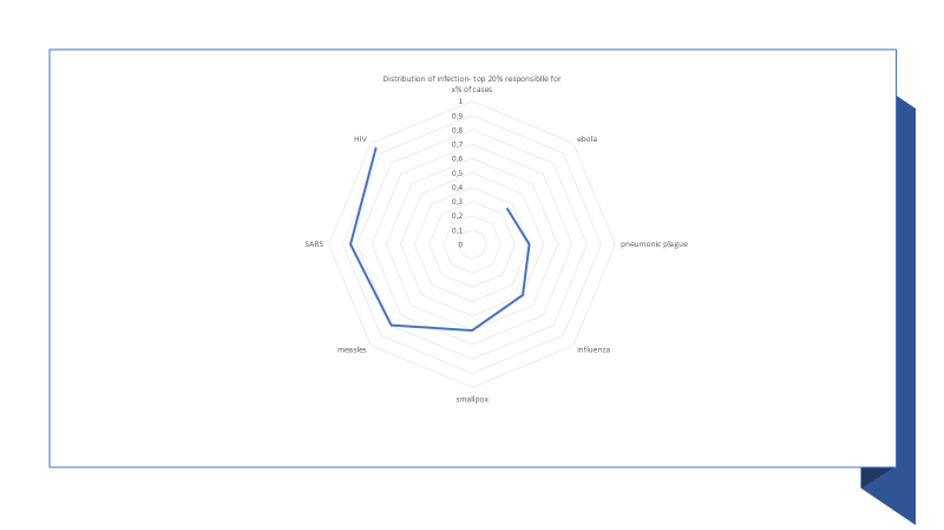
Source: Author own, Lloyd Smith et al., Litsearch

Getting the distribution skewness right for a disease has significant impact on the potential estimate of diffusion. For example, moving from a distribution such as observed for measles to one observed for Ebola, will more than double the number of infected cases by with super-spreaders (respectively, under-spreaders) achieve 2.3 (resp. 2) lower (resp. higher) infectious reach.⁷

At this time of writing, a scan of literature for COVID-19 has been unsuccessful, that would provide an assessment of the distribution type of secondary infections for the virus. Benchmarks for influenza suggest a skewed distribution, in the range of top 20% being accountable for 65% of secondary infections (Lloyd Smith et al. above). Using other cases, the distribution may be more homogenous, top 20% contributing 40% of secondary cases.⁸ Using those ranges, this means that compared to the mean $R_0$, we may have to discount the total diffusion by a correction factor, in the range of 40% and up to 70% if the distribution is skewed and (hopefully) closer to Pareto.

5. The emerging best guess picture for COVID-19: potential without control of up to 20 million fatalities worldwide

Back to Table of Contents

Four clusters of viruses

Table 2 provides a high level picture of epidemic difference per virus and injects the current range estimates for Covid 19. Four clusters emerge when looking at the table:

The “niche killer”: one notes that MERS, despite high fatality rate, for instance was a small outbreak, confined to Middle East, and with low and unequal reproduction rates among infected.
The “confined killer”: The Ebola outbreak was much more powerful but controlled to Africa.
The “global hitter”: The H1N1 virus has been typically spreading worldwide,…
The “serial killer”: but the 1918 flu had much lethal effects on infected and was more consistent in spreading towards secondary infections than the 2019 outbreaks.

Table 2: three « KPI » Metrics for different viruses (high level)

Year	Virus	Scope	Mean R₀	Top 20% contribution	Fatalities
1918	H1N1	Worldwide	1.8 to 2.2	40%	2%
2002	SARS	Asia	1.6 to 1.9	85%	9/10%
2003	Ebola	Africa	1.5 to 2.5	35%	55%
2009	H1N1	Worldwide	1.5	65%	0.2%
2012	MERS	Middle East	0.5	70%	30%
2019	COVID-19	Worldwide	1.3 to 2.0	40% to 70%	0.5% to 2%

Source: Author’s own computation based on WHO, Lancet, wikipedia, CDC, Nature

COVID-19: a global hit to control

If we look at the three figures on Covid 19, the virus falls into a solid global hitter. The mean range is similar to the low range of the 1918 H1N1 –but can be higher than in the 2009 outbreak; the fatality rate is likely half that of the 1918 outbreak but also at least twice the one to date in the 2009 pandemics. The evidence regarding the disparity of secondary contamination is not known to date, but taking the average of range for other influenza virus, we might be midway to H1N1 in 2009 and the Spanish flu by 2018.

Using all figure ranges as displayed in Table 3, and assuming an independent normal distribution of each KPI, we infer that the mode just below 20 million fatalities, with a standard deviation of about 5 million less or more casualities

Table 3: three « KPI » Metrics impact on likely covid 19 evolution

Range from	R₀ (*)	Skewness (*)	Fatality rate (=)	Total world pop (million)
Low	19%	0.3	0.5%	0.03% (2.5 million)
Mean	35%	0.5	1.2%	0.21% (18 million)
High	35%	0.7	2%	0.56% (48 million)

Source: derived from above figures, author’s computation

Note the crucial element of this table: this is the potential of the virus, if left freely to attack (of course unlikely, given the fatalities implied). But this is roughly more than 20 times the traditional burden of the normal, seasonal, flu at potential of 650,000 individuals, ($R_0$ of flu is 1.3; and fatality rate is tyipcally 0,1% as said earlier), and roughly 5 to 10 times, recent pandemic H1N1, in 2009, with $R_0$ at 1.5 and fatality rate at 0.2% (potential of 2 millions).

This potential in million deaths is caused among others by the multiplier nature, $R_0$, of contagion. But this is the reason why it is useful powerful to have active intervention by population and by government, to curb the spread the disease, with a mix of medical (antiviral and vaccine) and of non-medical actions (containment; border control, etc). The multiplier in this case plays the other way round; in the case of for instance H1N1 in 2009, the WHO has finally evaluated a total death toll of just below 300,000, that is, 15% of full potential.

As another example, the potential of SARS, despite high fatality rate, was restricted by its variance of contagion, and a pandemic restricted mainly to China (and some imports to US an Canada), at 6 million inhabitants worldwide. The final death case is less than 10,000, or a reduction of 99% of the potential. What made the case more controllable in the case of the SARS is three two things: symptoms like fever coincided with period of contagion, making people easily identifiable of being contaminated, and thus be put in quarantine. Furthermore ,the high rate of fatality made people naturally afraid of the virus, and hence, used a large plethora of self protective behavior. In the case of COVID-19, it looks like the latency period before symptoms are revealed may be at least 5 days, while a large number of cases may be mild, even asymptomatic, making the pandemic much more challenging to control.

This potential is not to be neglected and is to be the largest cause of deaths in the world for 2020 (see Table 4), or in the top of the list, under history of controlling pandemic influenza in the past.

Table 4: ranking of casualties, per 100,000 pop, worldwide estimates

Estimated mode Covid 19 (under no action)	210
Ischaemic heart disease	126
Stroke	77
Estimated mode Covid 19 (success rate control H1N1 , 2009)	31
Alzheimer's disease and other dementias	27
Trachea, bronchus, lung cancers	23
Diabetes mellitus	21
Diarrhoeal diseases	19
Tuberculosis	17

Source: author’s computation, wikipedia

Note: COVID-19 fatalities are higher among co-morbid patients, with diabetis, hearth diseases, etc. Thus, it has also extra effects on top diseases, not shown here

In our simulation, and taking the range of our estimates on the three parameters studied, we find that there is further only 1% chance that i will be « as low » as the 1957 H2N2, which already has double the number of fatal casualties of what has been seen from the worst normal flu epidemia. The « only good » news is that Covid 19 has only 1% chance to be as lethal as the Spanish flu, but a possible Black Swan is not to be excluded, as part of our range of scenarios, to define the danger of the disease.

6. A coordinated global action plan may be required

Back to Table of Contents

As the epidemy continues its course, it is thus critical to act in order to avoid the predictions set by the three current figures.

Multiple actions can be undertaken, like average social distancing measures of closing frequent and large interaction environments (reducing $R_0$), like spotting super spreaders (playing the skewness, or still by attempting to find good care and protection, playing on fatalities), with retrovirus might be more timely and a promising route.

As the world is more and more connected, all levers may have to be playing in the same time, and across the globe. If those levers play each to reduce 50% of the burden, the COVID-19 will look like a 1957 disease—an important pandemic, enough to remember that global management to contain lethal diseases is both necessary and successful. Hence, it is thus time to scale and synchronize efforts, versus too much wait. In a subsequent article, we will look at the likely economics of the pandemics, showing that economics add further fuel to the idea of correctly manage as scale against the spread of those types of viruses.

© Jacques Bughin. Written March 02; revised March 21. Comments more than welcome. All errors are mine. References listed as they are found in the text.

Hurbin, 2011, OECD report contribution to the project « Future Global Shocks », OECD. ↩
Vogel (2014). How deadly is Ebola?, ScienceMag. ↩
Mboup et al., (2006). HIV/AIDS, chapter 17 in Disease and mortality in Sub-Saharan Africa, EBRD/World Ban. ↩
Fan et al. (2018). Pandemic risk: how large are the expected losses, Bulletin of the World Health Organization. ↩
Kermack and McKendrick, (1927). A Contribution to the Mathematical Theory of Epidemics, Proceedings of the Royal Society. ↩
Lloyd Smith et al (2005). Superspreading and the eﬀect of individual variation on disease emergence, Nature. ↩
Brauer (2019). Early estimates of epidemic final sizes, Journal of Biological Dynamics. ↩
Hebert-Dufresne et al., (2020). Beyond $R_0$: the importance of contact tracing when predicting epidemics, ArXiv. ↩

1. Introduction

March 2

2. A history of scary viruses

3. What about influenza?

4. The three indicators that matter for COVID-19

Indicator 1. Fatality rate : Enough to take notice (range 0,5% to 2%)

Indicator 2. Reproduction rate: More a wide pandemic than a niche (adjusted \(R_0\) between 1.3 to 2, with mean at 1.9)

Indicator 3. Variance of reproduction. Super-spreaders likely the rule (Top 20% accounts for between 40% to 70% of secondary infections).

Accounting for super-spreaders versus limited spreaders.

5. The emerging best guess picture for COVID-19: potential without control of up to 20 million fatalities worldwide

Four clusters of viruses

COVID-19: a global hit to control

6. A coordinated global action plan may be required